Summary of Programme:

· Conducted customer churn analysis for Lloyds Banking Group. 
· Processed multi-source customer data to create 20+ structured features, standardised feature scaling, and cleaned noisy data.
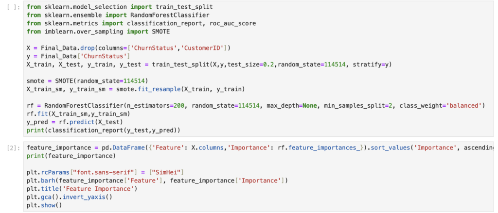
· Built a prediction system using a Random Forest classifier, resolved class imbalance through SMOTE oversampling.
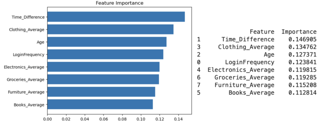
· Applied feature importance analysis to pinpoint top churn factors, delivering data-driven insights to reduce customer attrition risk.

What I have learned:

# I. Feature Selection and Engineering

1. Dimensionality Reduction Techniques
(1) Core Methods: PCA (Principal Component Analysis), t-SNE.
(2) Core Function: Alleviate the “curse of dimensionality” (high-dimensional data leads to poor model generalization and large computational load), simplify the feature space, and improve the training efficiency and generalization performance of the model.

2. Feature Importance Analysis
(1) Core Method: Ensemble algorithms such as Random Forest can directly output feature importance.
(2) Core Function: Precisely select highly predictive features, simplify the model structure while avoiding the loss of prediction accuracy and improving model interpretability.

3. Non-linear Feature Construction
(1) Core Method: Construct feature interaction terms and polynomial features.
(2) Core Significance: Make up for the deficiency that linear models (e.g., Logistic Regression) cannot capture non-linear relationships, and significantly improve the predictive ability of such models

# II. Algorithm Selection and Key Points

1. Logistic Regression
(1) Advantages: Simple model structure, efficient training, and extremely strong interpretability (can directly quantify the impact of features on results).
(2) Considerations: When processing high-dimensional data, it is necessary to combine L1 (feature sparsification)/L2 (outlier suppression) regularization to prevent overfitting.

2. Decision Tree & Random Forest
(1) Core Logic of Decision Tree: Take features as judgment nodes, branch layer by layer according to the “optimal splitting rule” (e.g., information gain, Gini coefficient) to complete binary classification/regression. The process is similar to making multiple-choice questions step by step, and finally falls to a unique conclusion leaf node.
(2) Core Logic of Random Forest: Construct multiple decision trees (each tree randomly selects part of the features and samples data randomly), and synthesize the results of all trees through “majority voting (classification)/mean value (regression)”.
(3) Advantages: Significantly reduce the overfitting risk of a single decision tree, be good at capturing non-linear relationships and interaction effects between features, and can directly output feature importance.

3. SVM (Support Vector Machine)
(1) Core Logic: Find the optimal hyperplane (the “separation line” in high-dimensional space) to separate data of different categories, and maximize the margin between the hyperplane and the nearest samples (support vectors) on both sides (the larger the margin, the stronger the model’s generalization ability).
(2) Advantages: Can map non-linear data to high-dimensional space through kernel tricks (e.g., RBF kernel, polynomial kernel) and convert it into a linearly separable problem.
(3) Considerations: Need to finely tune the hyperparameters C (regularization strength, controlling overfitting) and gamma (kernel function bandwidth, affecting the smoothness of the decision boundary).

4. Neural Network
(1) Core Logic: Simulate the hierarchical connection of human brain neurons, perform “multi-layer linear transformation + non-linear activation” on input features, extract the deep laws of data layer by layer, and finally output classification/regression results.
(2) Advantages: High accuracy when processing complex data patterns (e.g., high-dimensional images, time-series data).
(3) Considerations: Rely on a large amount of data and computing resources; need to prevent overfitting through technologies such as dropout (randomly discarding some neurons), batch normalization (stabilizing the training process), and early stopping (stopping training after reaching optimal performance).

# III. Model Evaluation and Tuning

1. Model Validation Methods
(1) Stratified K-Fold Cross-Validation:
· Core Logic: When splitting the dataset, ensure that the category proportion of each subset is exactly the same as that of the original dataset.
· Advantages: Avoid category imbalance of subsets caused by random splitting, especially suitable for imbalanced data scenarios such as customer churn prediction, and verify the model’s generalization ability more accurately.
(2) Bootstrapping:
· Core Logic: Resample data with replacement to construct multiple training sets and evaluate the model.
· Advantages: Estimate the distribution of model performance metrics (e.g., accuracy, F1 score), and analyze the variability and robustness of prediction results.
(3) Calibration Curve:
· Core Logic: Verify whether the predicted probability (or confidence) output by the model matches the actual occurrence frequency of results.
· Advantages: Optimize the model’s probability estimation ability and avoid decision-making errors caused by probability calibration deviation (e.g., misjudging high-risk customers).

2. Hyperparameter Tuning
(1) Core Logic: Hyperparameters are parameters manually set before model training (e.g., C of SVM, maximum depth of Decision Tree) and cannot be automatically learned through training. The goal of tuning is to traverse and select the optimal combination of hyperparameters to maximize the model’s generalization ability on new data.
(2) Basic Methods: Grid Search (exhaust all preset parameter combinations, high accuracy but extremely high computational cost), Random Search (randomly sample parameter combinations, higher efficiency and performance close to Grid Search in most scenarios).
(3) Advanced Methods: Bayesian Optimization (predict the optimal parameter region based on probabilistic models and conduct targeted search), AutoML tools (automatically complete the entire tuning process).

3. Algorithm Adaptability Selection
(1) Simple algorithms (Logistic Regression, Decision Tree) have strong interpretability and low deployment cost, but limited prediction accuracy.
(2) Complex algorithms (GBM, XGBoost, Neural Network) have high prediction accuracy and can process complex data, but weak interpretability and high computational/deployment cost.
(3) The core basis for selection is the business trade-off between “performance and interpretability” (e.g., prioritize interpretability for regulatory scenarios and prioritize performance for accurate prediction scenarios).

4. Evaluation Metrics for Imbalanced Data: 
Traditional accuracy metrics are misleading, and the following metrics should be prioritized
(1) Precision and Recall:
· Precision = True Positive / (True Positive + False Positive), which measures “the proportion of true positives among results predicted as positive”.
· Recall = True Positive / (True Positive + False Negative), which measures “the proportion of true positives correctly identified among all actual positives”.
· The selection basis should combine business costs (e.g., prioritize Precision if the cost of false positives is high, and prioritize Recall if the cost of false negatives is high).
(2) F1 Score: The harmonic mean of Precision and Recall, whose core function is to balance the performance of both. It is suitable for scenarios where the error costs of false positives and false negatives are similar.
(3) ROC-AUC: Measures the model’s ability to trade off True Positive Rate and False Positive Rate under different decision thresholds. The higher the score (between 0 and 1), the stronger the model’s overall ability to distinguish positive and negative classes, which is not affected by threshold selection.
(4) Confusion Matrix: Intuitively decompose the four types of prediction results: “True Positive, False Positive, True Negative, False Negative”.

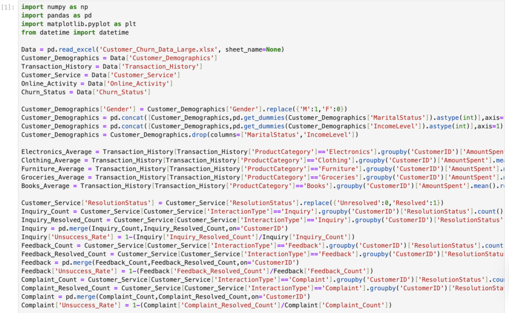
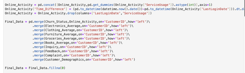
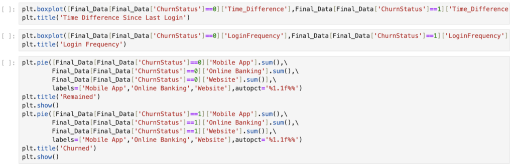
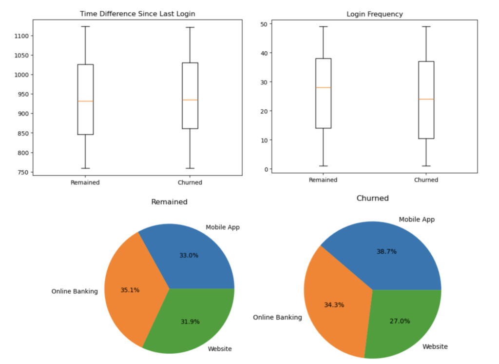
Screenshot for Document 1: